Aerospace Finite Element Methods
What is Finite Element Analysis
- The FE method involves breaking a structure into several elements (pieces of the structure)
- Describing the behavior of each element in a simple way.
- Elements are then reconnected at nodes (nodes hold elements together list glue)
- The process results in a set of up to several thousands of simultaneous equilibrium equations, which require a computer to solve.
Brief History of FEM
- Courant (1943) first developed FEM to solve the problem of torsion of a hollow shaft with a rectangular cross-section.
- Subdivision of cross-section into small triangular sub-sections with linear approximations for displacement over each triangle.
- Assembling of all triangles into a matrix for the whole cross-section, he derived a simple solution for a up-to-date unsolvable problem.
- Work was not discovered until 1960, when the name “finite elements” was coined by Clough at University of Berkeley, USA.
- By late 1980s, method had been implemented into many commercial finite element packages, namely NASTRAN, ABAQUS, ANSYS, STRAND, LS-DYNA, PAM-CRASH, etc.
- Is used on all kind of computers from PC to supercomputers with parallel processing.
- For aerospace companies (Airbus, Boeing) and research teams, ABAQUS is often the main commercial software package.
Finite Element Method
- The behavior of complex structures cannot be solved using analytical methods.
- Finite Element Analysis (FEA) is a numerical method that breaks down a structure into discrete elements.
- The behavior of each discrete element can be calculated.
- The global response of the structure is observed by combining the results of each finite element.
FEA can solve a variety of problems
- Deformation analysis
- Stress Analysis
- Natural Frequencies
-
Buckling Analysis
- Allows for the analysis of:
- Complex geometries
- Complex situations (constraints, boundary conditions)
- Various physics (structural, thermal, acoustics, etc)
Analysis Types
What separates Engineers from Scientists:
Scientific Analysis:
- As accurate as possible
- Looks at future technical applications
- Driven by a want to just expand knowledge
Engineering Analysis:
- As accurate as required
- Looks at Current technical applications
- Is commercially driven
Approximations in FAE
- An object is manufactured out of metallic material. Any metal consists of atoms in a crystal structure. Atoms are discrete, not continuous.
- Mathematical models solve structural and vibrational problems assuming that the object acts as continuous object.
- Mathematical models provide useful solutions to engineers and scientists through methods of differential and integral calculus.
- Only simple mathematical problems can be solved analytically.
- Complex equations are solved through numerical methods.
Numerical Methods
- Mathematical model is solved approximately
- Final Difference Method
- Closely related to the solution of mathematical equations.
- Often used for systems of time-dependent partial differential equations (e.g. heat transfer problems diffusion problems).
- Not well suited for complex boundary conditions.
- Finite Volume Method
- Flow problems with complex boundary conditions (heat transfer, diffusion problems)
- Finite Element Method
- Ideally suited for models with complex boundary conditions
- Mixtures of materials
- Mixtures of different structural shapes (trusses, beams, thin shells, solids)
- Used in all fields of engineering and science today
- Methods differ by how they divide the space to be analyzed.
Truess Structures
Truss Structures consist of truss members, i.e. bars that can be loaded only axially. There is no bending allowed, In practice, the connection of trusses in the joints has to be such that the requirement of axial loading can be satisfied.
Why Start with Truss Elements?
- Truss elements are often used in constriction.
- Trusses belong to the class of skeletal structures and consist of members connected at joints.
- Skeletal structures can be analyzed with a variety of hand-oriented method of structural analysis: displacement and force methods.
- Skeletal structures can also be analyzed by computer-oriented finite element methods (FEM).
- FEM will give the exact same answer as your hand calculation.
- Therefore, truss element structures are the ideal choice to introduce computer-oriented terminology and explain the fully-automated numerical solution method.
Derivation of the Stiffness Matrix
Three methods to be introduced:
- Direct observations (Trusses)
- Unit displacement method (Trusses and beams)
- Method of virtual work (All Elements)
Direct Observations
Bar/Truss elements
- 1D truss element defined by length L, cross-section A and stiffness E
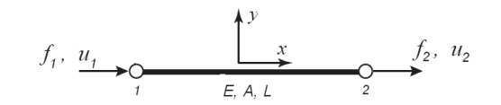
-
Truss Stiffness: \(k = {EA \over L}\)
- Equivalent spring stiffness
- Note $k = {f / \delta}$,
- So, force is $k \cdot \delta$
- $u_2 - u_1 = \delta$
- The element is static and so the sum of forces is zero hence $f_1 =-f_2$
- So, Force:
- Matrix form:
gives,
\[\begin{bmatrix} k & -k \\ -k & k \end{bmatrix} \begin{bmatrix} u_1 \\ u_2 \end{bmatrix} = \begin{bmatrix} f_1 \\ f_2 \end{bmatrix} \Rightarrow K^e .u^e = f^e\]e is the element number. So what part of the structure we are considering. We have to calculate this for each element in the structure to get a full picture.
- K: Element stiffness matrix, u: displacement vector, f: force vector
- Equilibrium: $f_1 = -f_2$, but system is free to move (no boundary conditions)
Stiffness in Stuctures
A material has a value for stiffness which is given by Youngs modulus. For a structure which will act differently depending on its geometry such as length and cross-sectional area we can use Hooke’s law to calculate a structural spring constant.
\[{F \over \delta} = {EA \over L} = {K}\]For a structure with multiple degrees of freedom we need to consider the stiffness in the various directions it can be displaced.
So for a structure with 3 nodes we need to consider the displacement at node 1 due to a force at node 2, also the displacement at node 1 due to a force at node 2 and so on. We denote this with:
u: displacement F: Force
so,
\({F_2 \over u_1 } = K_{21}\) Which is the displacement at node 1 due to a force at node 2
We use a matrix to represent all these k values for the various relevant stiffness values.
Method of Virtual Work
Definition: Virtual displacement is a change in the configuration of a system as the result of any arbitrary infinitesimal ‘admissible displacement $\delta u$’ (change of the coordinates ) consistent with the forces and constraints imposed on the system at a given instant of time.
-
Most general method (less intuitive), which is used for derivation of stiffness matrices for more complex element types (shells, solids).
-
Derivation for truss elements not necessary (can be done by unit displacement method), but demonstrates the principle.
-
It is a thought displacement, not a real one, once could say an “as if displacement, or “what happens if” displacement.
-
Method of virtual displacement can be traced to Aristotle (384 — 322BC) and was mathematically formulated by Bernoulli (1667-1748).
Method
Truss Elements
- Truss under virtual end-displacement $\delta W_{\mathrm{e}}=\delta W_{\mathrm{int}}$
- Virtual work by external (end) forces \(\delta W_{\mathrm{e}}=f_{1} \delta u_{1}+f_{2} \delta u_{2}\)
- Virtual work of internal forces (elastic deformation): \(\delta W_{\text {int }}=\int \delta \varepsilon \sigma d V=\int_{0}^{L} \delta \varepsilon E \varepsilon A d x=\delta \varepsilon . E A L \varepsilon \quad \text { with } \quad \varepsilon=\frac{\left(u_{2}-u_{1}\right)}{L} \Rightarrow \delta \varepsilon=\frac{\left(\delta u_{2}-\delta u_{1}\right)}{L}\)
- Force equilibrium: \(E A L\left[-\frac{\delta u_{1}}{L}\left(\frac{u_{2}-u_{1}}{L}\right)+\frac{\delta u_{2}}{L} \frac{\left(u_{2}-u_{1}\right)}{L}\right]=f_{1} \delta u_{1}+f_{2} \delta u_{2}\) \(\Rightarrow f_{1}=\frac{E A}{L}\left(u_{1}-u_{2}\right) \quad \text {and} \quad f_{2}=-\frac{E A}{L}\left(u_{1}-u_{2}\right)\) This gives: \(\frac{E A}{L}\left[\begin{array}{rr}1 & -1 \\ -1 & 1\end{array}\right]\left[\begin{array}{l}u_{1} \\ u_{2}\end {array}\right]=\left[\begin{array}{l}f_{1} \\ f_{2}\end{array}\right]\) Same result as derived earlier where $k = {EA \over L}$